Some Examples of how HPD Supersedes What Exists
(i) Existing Practices
(ii) Comparing Results from HPD_VA to What Exists
(iii) Comparing Taguchi Methods (TM) to HPD_Opt (& HPD_OW)
Although HPD_VA is the most important suite and contains most of the fundamental advancements, in (ii), we’ll only need to show 2 examples to give enough flavor, but in (iii) for Design Optimization, a fuller discourse is given because there is so much to clarify; thus, we’ll point out (a) TM’s major problems and (b) how HPD_Opt far supersedes TM. (This is a long webpage for those who like details; others could skimp through for the flavor.)
(i) Existing Engineers’ Practices for Addressing Variability
- For Variability Analysis (e.g., for tolerancing, failure analysis, obtaining Output variability, . . .):
Monte Carlo (+ variants); Form/Sorm-based software; RSS (mostly inappropriately); Worst Case; . . .
- For Design Optimization:
Some use Taguchi Methods; many use ad hoc DoEs; some use iterative processes
On Comparing What Exists to HPD’s Capabilities
- For Variability Analysis: Much on other pages has covered how HPD_VA leapfrogs over Monte Carlo and supersedes existing Sensitivity Analysis techniques, thus we’ll show just 2 examples in (ii)
- For Design Optimization: We’ll just compare Taguchi Methods (TM) to HPD_Opt (& HPD_OW) in (iii) below.
Important:
- TM optimizes for Robustness
- HPD optimizes for Robustness AND Latitude (latter is much more important; meaning given in (iii)’s textbox)
(ii) Examples Using HPD_VA
1. Computing output distribution, failure rates, and reuse outputs for inputs:
For the well-known cantilever beam equation, z = g(X),
with a set of specific input distributions,
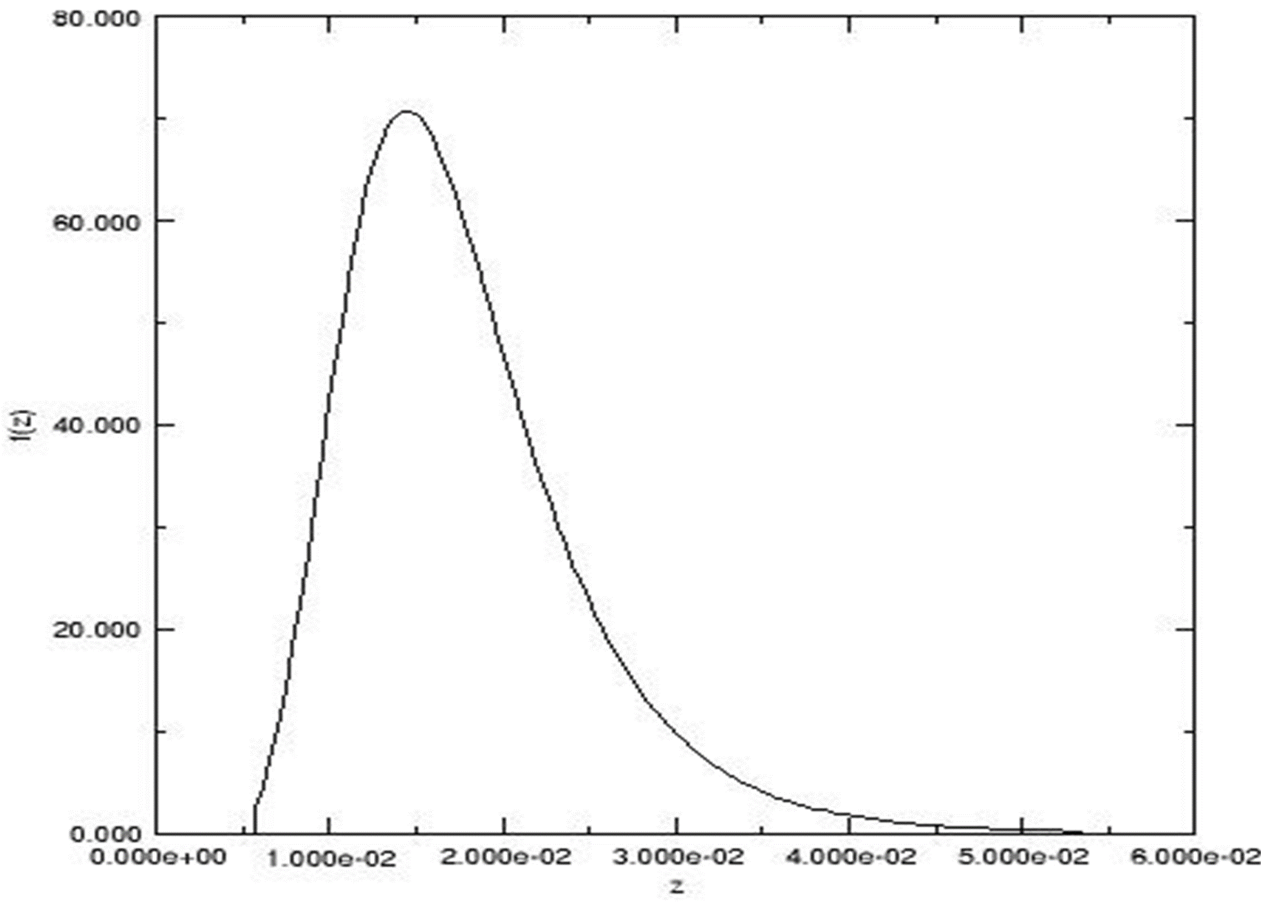
the resulting (“exact”) density distribution, fz(z), is:

Another tool in HPD_VA directly computes the Prob(Fail) for a given Failure Criterion (FC) or a set of FCs. For the beam example shown, the FC z > .04 gives
Prob(Fail) = .01054
(Prob(Fail), of course, is just 1 point on the cum distribution which is outputted with the density.)
( For > 1 FC, need za, zb, . . . )
Note:The tool for computing distributions also conducts our advanced Sensitivity/Contribution Analysis. Then it uses the High-Contributors (HCs) to compute the output density & cum distributions, and adjusts for the % contributed by the omitted non-HCs.
The output distributions are, of course, usable as input distributions in next level relationships (i.e., models).
2. Comparing results from using HPD’s Correct Sensitivity/Contribution Analysis (SA/CA) vs. that from existing SA/CA tools:
(Only very compacted results are given here; no graphics are shown.)
HPD’s SA/CA includes treating Cross-Term Effects and NUness (to be explained at talks, in the tool, and in Volume 1 of Series
From an actual application: Motion Control of an Imaging System.
The engineer-derived equation had 17 RVs. (This was not a multi-level model)
Impact on Density & Prob(Fail)
| 2 Steps (due to 17 RVs) | From HPD | From Existing Techniques/ Tools |
| 1a. From SA/CA Result | 4 High Contributors (HCs) | 3 HCs |
| 1b. From output density using the HCs (The density shapes differed a lot!) |
(zmin, zmax) = ( – 0.697, 0.632 ) |
(This part of computation used HPD) (zmin, zmax) = ( – 0.406, 0.390) |
| 2. Prob (Fail) for z > 0.45 | Prob(Fail) = 0.0176 |
(This part of computation used HPD) Prob(Fail) = 0 (grossly wrong!!) |
(Not given here are many other examples such as structuring “Total Models” for (a) quasi-hierarchical relationships or (b) sequential ones.)
(iii – a) Some Major Problems with Taguchi Methods (TM)
- If there are Interactions, and those hadn’t been pre-identified, the optimal point by using one OA (º Orthogonal Array) can differ from that by using another OA!! (See reference under Announcement.) Mostly, TM results are valid only for problems with no interactions, but then the optimization process could be far more simplified! Also, Basic fallacy exists from using S/N ratios (see same reference).
- TM needs a 2-step process to find the optimal point that meets the Target mean: Parameter Design and using an Adjustment Parameter, all without having properly considered Variability, and certainly not probability distributions of any type. It then uses Tolerance Design (the 3rd step) to meet the stochastic target, typically with too tight tolerances. Thus, TM greatly sub-optimizes (to compensate for not quite the optimum and the 3-step process). (This is without user’s realizing it!)
- Experimentally, it cannot handle Internal Noise, the most important part of meeting a Stochastic target!!
- It cannot find Operating Windows which is extremely important for attaining Latitude (meaning is given in next textbox) — even more important than finding the most Robust point!
- It cannot treat any case where there are > 1 performance characteristic
Engineers use TM only because till now nothing else has existed for Optimizing for Robustness, though they do not fully understand TM and its significant shortfalls. … Also, they use smaller OAs to reduce confusion.
(iii – b) HPD’s Stochastic Optimization (SO) Tools: HPD_Opt & HPD_OW
(Note: It is not possible to do justice to HPD’s SO in one textbox of info, thus this is skeletal at best.
Even so, there is so much detail. It is meant for the serious reader; others could glance just to get the “flavor.”)
- HPD‘s SO tools: HPD_Opt (for 1 z) and HPD_OW (post-processor for > 1 z)
- HPD_Opt (uses HPD_VA as compute engine, thus uses Probability Distributions!):
- Has 36 combos of possible situations in basic subpaths:
[Target Types] x [FF, Mixed, CC] x [Analytical; Lab (µ & σ); Lab µ] x [σ; Spread**]
Note: Internal Noise is always covered (!); For Lab cases, External Noise is covered by the Lab (µ & σ) subpath;
(** For non-Normal distributions, Spread is equivalent to 6σ span of Normal Distribution)
-
- The (Robustness) Optimization Criteria are (can choose σ or Spread, or both):
min σ; max | µ |/σ; min Spread; max | µ |/Spread
-
- TM’s capabilities are included in (part of) only 2 of HPD’s 36 combos!!Also Important: Relative to TM, HPD:
-
-
- Obtains results far more appropriately (in 1 step), thus does not sub-optimize
- Takes care of interactions (full, partial, or none)
- Determines the Operating Window (region where target is met!), a larger size indicates having Latitude!
- Re. Operating Windows (OWs):
- They are obtained Stochastically, thus are Stochastic OWs, or SOWs
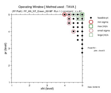
- A very simple SOW from a sample run:
- They are obtained Stochastically, thus are Stochastic OWs, or SOWs
-

For a multi-dimensional Optimization Region, viewable (& printable) are 2-D slices with the corresponding SOW in each slice. Results first indicate sizes of the SOWs in the slices; the slice with the largest SOW as best choice. But a SOW that is too small means inadequate Latitude. (Methodology easily instructs what to do if this occurs or when no slice has a SOW.)
In this slice of Optimization Region, the SOW is the upper right area (“covered” by the black solid circles). The optimal point is point in the thicker red circle or in the thicker green square. Nearly optimal points are in lighter circles/squares . . . . Results include formatted datasets of useful info at many relevant points. . . . Much more can be discerned from the results (e.g., most Robust point may not be best, as in this case!).
- HPD_OW: Very important; many problems have > 1 z. Run HPD_Opt for each, then apply HPD_OW to the set!
- HPD_VA’s tools & the HPD Methodology can be used to support the SO process, if needed.
- All results & process are in simple engineering lingo, thus simplifying understanding of their problem & process.

